An MVP You Can Finish: Scoping Fabric v0.1

Chapter 1 ended on April 7, 2026, with a folder of RFSoC and SDR tools becoming the first commit of a new repository. This chapter covers April 7 to 8. Version 0.1.0 was tagged on April 8, 2026, one day after that first commit. The history for those two days is short: one commit on April 7 and three on April 8.

A one-day gap between the first commit and the first version sounds like a sprint. What made it possible was scope. This chapter is about what that first version was allowed to do, what it was not, and the bit of physics that explains why the core idea, propagating rates and types through a graph, was worth building first.

The commit that became v0.1.0 described itself as the "Complete RF System Design Configurator (Phases 3-6)". Two things in that message matter. The first is the name: at this point the product was the Apexia RF System Design Configurator, not Fabric. The second is the word phases. The work had been broken into numbered phases before it was built, and the version tag marked the point where a planned set of them was done.

That is the habit I would keep from this chapter if I kept only one. I planned each subsystem in a written spec and an implementation plan before building it. A plan with numbered phases gives you a finish line you can see. Without one, an MVP drifts toward whatever is interesting that afternoon.

The README from the v0.1 to v0.2 period describes the core. At its centre was a drag-and-drop node graph with 42 block types across 5 categories: RF, DSP, sensing, clock and I/O. Around it:

• Propagation: sample rates, data types and centre frequencies flowed along the edges in real time, so every block knew what it was receiving.
• Typed ports: colour-coded and type-checked, with five kinds (IQ, real, clock, trigger and control), so every connection was type-checked.
• Composite channel nodes for RX and TX channels.
• Editing basics: undo and redo, copy and paste, snap-to-grid.
• A scope block to look at the signal at a point in the chain.

The connection to real hardware came early too. From early on, Fabric could export Vivado TCL that matches the CASPER yellow-block parameter naming, export casperfpga Python scripts, capture snapshots with IQ deinterleave, configure the NCO, decimation and Nyquist zone at runtime, configure the PLL, and run a multi-tile synchronization wizard. That was the point of Chapter 1: the model you checked should be the configuration you build, without retyping it into a wizard.

The cut list is easier to see in hindsight, because the history shows when each missing piece finally arrived. Three things that Fabric has today were not in the MVP:

• No installers or desktop packaging. That work started on April 25.
• No code generation for USB SDRs. That arrived in August.
• No documentation site. That came in late July.

Each of those is a real feature, and each is a trap for a first version. Packaging only matters once there is something worth installing. Code generation for a second family of radios multiplies the surface you have to keep correct. A documentation site describes a product whose shape is still moving. None of them tests the central bet, which was simple: if rates, types and frequencies propagate through a model of the chain, the model can catch mistakes before hardware does. In hindsight, the MVP tested that bet and connected it to the toolflow I already used. Everything else waited.

Propagating sample rate and data type sounds like bookkeeping. It is more than that, because a few numbers at a node, the converter's word length and the rates in and out, set a ceiling on the signal quality you can get there. The first of those ceilings is the familiar one. An ideal $N$-bit converter with full-scale range $\pm 1$ has a step size $\Delta =2/2^N$. If the quantization error is spread evenly across one step, its power is ${\Delta }^2/12$, and it is close to white across the band from 0 to $f_s/2$. That picture of quantization noise as a uniform, broadband error, valid for fine quantization of a busy signal, goes back to Bennett 1948. A full-scale sine has power $1/2$, so the ratio is:

The second ceiling is where the graph earns its keep. Because the quantization noise is spread over the whole Nyquist band, a filter that keeps only a bandwidth $B$ keeps only a fraction $2B/f_s$ of the noise. Decimate by $D$ to an output bandwidth $B=f_s/(2D)$, and the ceiling rises by the processing gain:

So a block in the middle of a chain can only state its ceiling if it knows the converter's word length, the rate it receives, and the rate it emits. That is exactly what the graph propagates. A tool that carries rates and types along every edge is in a position to tell you the SNR you are entitled to at every node, and to show you when a later block has thrown some of it away. The same rule lives inside Fabric itself: its test signal generator models converter noise with the ideal $6.02N+1.76$ dB rule.

FS 2.4576 GSPSADC 12 / 14-BIT IDEALFIR KAISER, POLYPHASESIM 16 TONES PER POINTSOURCE COMPUTED + SIMULATION

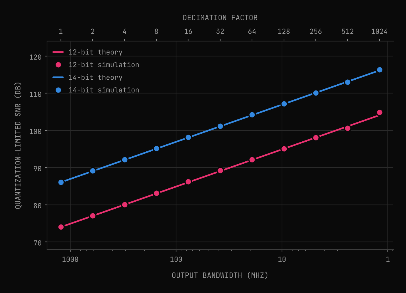
At 2.4576 GSPS the Nyquist band is 1228.8 MHz wide. Over that full band, an ideal 12-bit converter is limited to 74.0 dB and a 14-bit converter to 86.0 dB. Decimate by 8 to a 153.6 MHz band and those ceilings rise to 83.0 dB and 95.1 dB. Decimate by 64 to 19.2 MHz and they reach 92.1 dB and 104.1 dB. At a decimation of 1024, a 1.2 MHz band, the processing gain is 30.1 dB and the ceilings are 104.1 dB and 116.1 dB.

One comparison is worth stating plainly: a 12-bit converter decimated by 64 has a higher quantization ceiling (92.1 dB) than a 14-bit converter used over its full Nyquist band (86.0 dB). Bits and bandwidth trade against each other, and the exchange rate is fixed by the formula. That is a design decision you want to see at the node where you make it, not discover later.

The simulation checks the formula rather than assuming it. Each marker quantizes a full-scale sine at a random frequency between 0.2 and 0.45 of $f_s$, passes the quantization error through a polyphase FIR with its cutoff at the new Nyquist frequency, and averages the in-band error power over 16 tones. For decimation up to 256 the markers sit within 0.16 dB of the lines. At the narrowest band the 12-bit case drifts by 0.76 dB, because the error from quantizing a pure sine is really a set of discrete spurs, and in a 1.2 MHz band only a few of them land inside. The formula describes white noise; a clean tone is not quite that.

These are ceilings, not predictions. A real converter adds thermal noise, clock jitter and distortion, and real filters have finite stopbands. But a ceiling is still useful. If a block downstream reports less than its ceiling by a wide margin, something between the converter and that block is worth a look.

The first version had a scope block. Chapter 3 covers what happened to it from April 8 to 10: two-dimensional scope views, a shared catalog of window functions so that every view and block measured with the same definitions, and how a probe shifts what you ask of a design. You can try the current version of Apexia Fabric in simulation today.