The Probe Changes the Question: Scope Views and One Window Catalog

Chapter 2 ended on April 8, 2026, with version 0.1.0 tagged and a scope block in the graph. This chapter covers April 8 to 10. The history for those three days reads three commits on April 8, five on April 9, and 42 on April 10. Not all of April 10 was about the scope; the next two chapters pick up the rest of that day. This chapter follows the scope work.

Once you can probe any point in the chain and see the signal, the question you ask of a design changes. You stop asking whether the chain is wired and start asking whether it is right. That second question only has an answer if every view measures the same way, which is why a shared catalog of window functions arrived in the same week as the views themselves. This chapter is about both, and about the physics that made the catalog necessary.

On April 9 two things landed. The first was a set of two-dimensional scope views: response maps across two dimensions, and angle maps for the beamformer. The second was a centralized window catalog, one place where every window function is defined. On April 10 the signal analyzer and the block schemas moved onto that shared catalog, and the 2D heatmap views gained physical units.

Today Fabric's scope has seven views in total: spectrum, time, IQ constellation, waterfall, and the three 2D views. Its spectrum analyzer shows levels in dBFS with a reference level and dB per division, averaging, max and min hold, peak and delta markers, and a choice of 11 window functions. That is the feature list of a bench instrument, and a probe that reads like an instrument invites you to measure with it, not just look.

Physical units on the heatmaps belong to the same idea. A map without units tells you the chain produced something. A map in physical units tells you whether it produced the right thing. Before the probe, the useful question was whether the rates and types propagated without a conflict. After it, the question was whether the tone sat where the frequency plan said, at the level the gain budget said. That is a harder question, and it needs a ruler you trust.

A spectrum view takes $N$ samples, multiplies them by a window $w[n]$, and computes a discrete Fourier transform. The DFT only evaluates the spectrum at $N$ frequencies, the bins, spaced $f_s/N$ apart. A tone that falls exactly on a bin lands in one bin. A tone that falls between bins does not, and the window decides what happens to it. Harris 1978 is still the standard account of this, and it gives the figures of merit used below. The figures here are computed from the window samples, not copied from its tables.

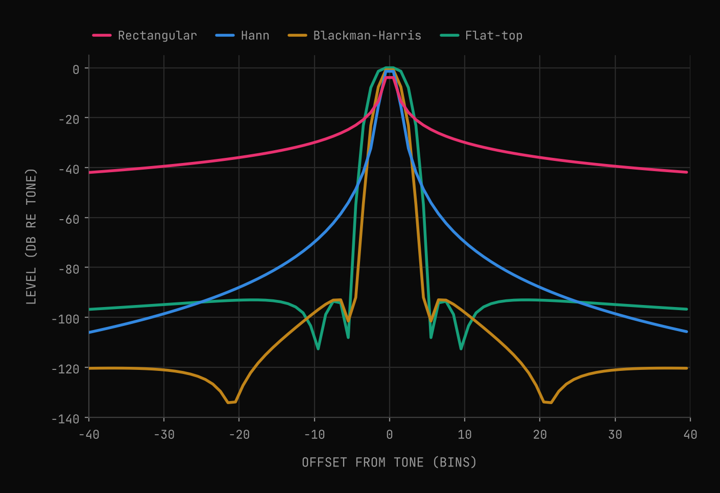
The first figure takes the worst case: a complex tone exactly halfway between two bins, at bin 256.5 of a 1024-point DFT. Each window is scaled by its coherent gain $\sum w[n]$, so 0 dB is the level a tone of the same amplitude would read if it sat on a bin. The plot shows the bins a probe would draw, from 40 bins below the tone to 40 above.

DFT N = 1024TONE BIN 256 + 0.5SCALE 0 DB = ON-BIN TONEWINDOWS PERIODIC; SCIPY FLAT-TOPSOURCE COMPUTED

Three effects are visible in that plot, and each one changes a number a probe reports.

Leakage is the skirt. With no window at all (rectangular), a tone between bins spills into every other bin: 39.5 bins away it still reads $-41.9$ dB. Any weaker signal in that range is buried under the skirt of a stronger one. Hann brings the same point down to $-105.7$ dB. Blackman-Harris and flat-top keep the far sidelobes about 92 dB or more below the tone. The price is a wider main lobe: the first null moves from 1 bin (rectangular) to 2 (Hann), 4 (Blackman-Harris) and 5 (flat-top).

Scalloping loss is the drop in the peak. A tone halfway between bins reads low by an amount that depends only on the window:

For the four windows that is 3.92 dB (rectangular), 1.42 dB (Hann), 0.83 dB (Blackman-Harris) and 0.01 dB (flat-top). The same half-bin tone therefore reads 3.91 dB apart depending only on whether the view used a rectangular or a flat-top window. That is why flat-top windows exist: they trade resolution for an amplitude reading that hardly depends on where the tone falls.

Equivalent noise bandwidth is the cost on the other side. A window that widens the main lobe also widens the band of noise each bin collects. Measured in bins, it is:

The second figure plots each window's highest sidelobe against its ENBW. The dots come from the formula; the crosses come from a seeded Monte Carlo that windows 400 records of complex white noise and measures the mean power per bin against an on-bin tone. The two agree within 0.73 % for every window.

DFT N = 1024SIDELOBE 64X ZERO-PADDEDMONTE CARLO 400 NOISE RECORDSSEED 20260409SOURCE COMPUTED + SIMULATION

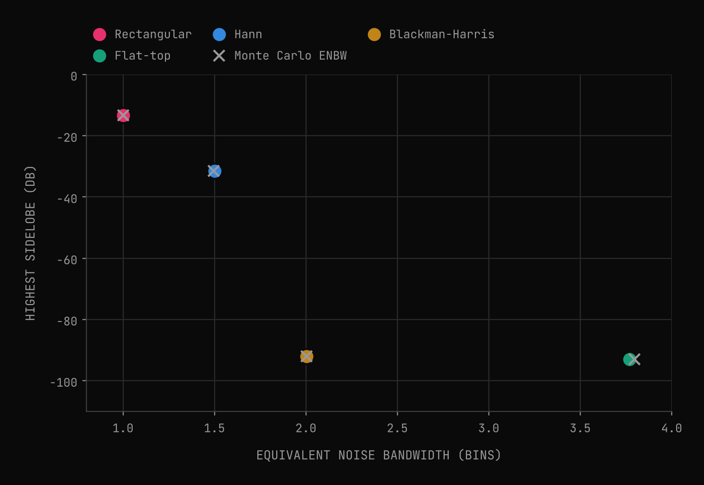
Read left to right, it is a price list. The rectangular window costs nothing in noise bandwidth and gives $-13.3$ dB sidelobes. Hann costs 1.500 bins (1.76 dB) for $-31.5$ dB. Blackman-Harris costs 2.004 bins (3.02 dB) for $-92.0$ dB. Flat-top costs 3.770 bins (5.76 dB) for $-93.0$ dB, and spends the extra bandwidth on a flat peak rather than lower sidelobes. No window wins on every axis; each is a choice about what you want to read accurately.

Put those numbers next to each other and the case for a shared catalog makes itself. Suppose the spectrum view uses Hann and a block that estimates a noise floor uses Blackman-Harris. Feed both the same white noise, normalize both to a tone, and their per-bin noise floors differ by 1.26 dB. Neither is wrong. They are measuring with different rulers. Now add a tone between bins, and the amplitude readings differ too, by an amount that moves as the tone moves.

A design tool that reports a level in one view and a different level for the same signal in another loses the trust that makes a probe worth having. So on April 9 the window definitions moved to one place, and on April 10 the signal analyzer and the block schemas were moved onto it. After that, every view and every block that used a window used the same definition of it. When two readings disagree, the disagreement is about the signal, not the arithmetic.

The same discipline shows up in the earlier post on digital down conversion: a number is only useful if you know how it was measured. A window is part of the measurement, so it belongs in one definition, not in each view's private copy.

April 10 had more in it than the window catalog. Chapter 4 covers the next part of that day: a written design spec for a System Architect, and a Python core with a system model of nodes, links and groups, plus timing, antenna and FPGA resource models. You can try the current scope views in Apexia Fabric in simulation today.