Throwing Away the First UI: A Rewrite, Plan by Plan

Chapter 4 ended on April 10, 2026, with a Python core for whole systems and a FastAPI service in front of it. The same day, something else started: a new front end. This chapter covers April 10 to 18. On April 18 the first interface was retired, and the repository tag `pyqt-final` marks its last state.

The first UI was PyQt, with matplotlib for the plots. It worked. This chapter is about why I replaced something that worked, how a written plan per subsystem made an eight-day replacement possible, and the piece of physics hiding in one of the views that was ported along the way: the live waterfall, which is a short-time Fourier transform and therefore a trade between time and frequency that no setting removes.

On April 10 a Vite, React, TypeScript and Tailwind front end was scaffolded. Three things went into it on the first day: brand tokens from the Apexia design system, a React Flow canvas for the system view, and TypeScript interfaces mirroring the Python models.

That last item is the one that explains the rest. Chapter 4 described a core with project, system, antenna, hardware, chain and frequency endpoints behind HTTP. Once the models live behind a service, a user interface is a client of that service. TypeScript interfaces that mirror the Python models are the contract between the two. Any interface that speaks that contract can draw the models; an interface that predates it has to be adapted to it.

The system view was the other pressure. Nodes, links and groups want a canvas built for graphs, and the new front end started with one. Keeping two interfaces alive, each needing every new feature, would have doubled the cost of everything that came after. One of them had to go, and the one built on the contract was the one with a future.

A rewrite of a working tool usually fails in one of two ways: it never reaches parity, or it reaches parity on the features someone remembered and quietly drops the rest. The defence against both was the same habit as in earlier chapters. I planned each subsystem in a written spec and an implementation plan before building it. Plan 2, the React front end, had been written on April 10 alongside the plan for the core. The plans that followed, in the order they appear in the history:

• April 12: Plan 4, the chain editor core, a React port of the PyQt block editor. Plan 5, the scope probe live view.
• April 14: Plan 7, export.
• April 15: Plan 6, composites and drill-in.
• April 16: Plan 8, PyQt retirement, with separate parity plans for the main window and the scope.
• April 18: the PyQt UI retired, tagged `pyqt-final`, and the PyQt tutorial scripts moved to `tutorials/`.

Plan 8 is the one I would point to. Retirement was its own plan, with parity written down for the two places where the old UI carried the most weight: the main window and the scope. The old interface was not switched off when the new one felt ready. It was switched off when a written list said the new one did what the old one did. And the last PyQt state was tagged rather than deleted, so nothing it knew was lost.

The commit history shows the pace that bought. April 2026 closed with 316 mainline commits on 12 active days, and 274 of them fall between April 10 and April 18. The busiest day was April 11, with 63.

MONTH APRIL 2026TOTAL 316 COMMITSAPR 10 TO 18 274SOURCE FABRIC GIT HISTORY

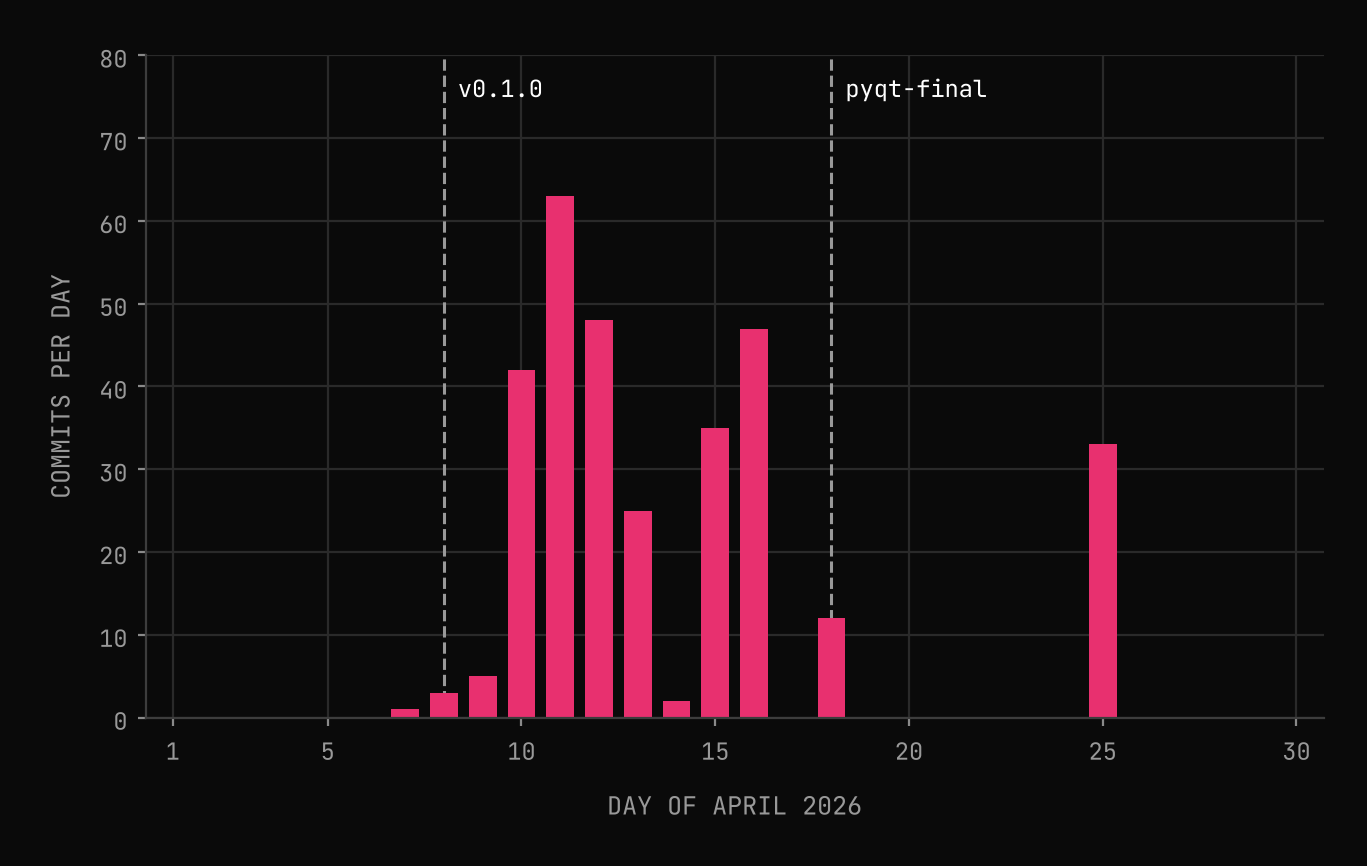
The shape matters as much as the total. The work comes in runs of days, with a near pause on April 14 (two commits, the day the export plan appears) and none at all on April 17. The single bar on April 25 belongs to the next chapter.

Plan 5 was the scope probe live view, and the scope's waterfall is a good example of a view that looks like a picture and is really a measurement with a choice baked into it. A waterfall cuts the signal into frames of $N$ samples, windows each frame, and takes a discrete Fourier transform of it. That is the short-time Fourier transform:

Two resolutions fall out of $N$ and the sample rate $f_s$. The bins are $f_s/N$ apart, and each frame looks at $N/f_s$ seconds of signal:

The product is fixed. Halve the window and you double the time detail and halve the frequency detail. Overlap is the setting people reach for to escape this, and it does not: it adds frames, but each frame still averages over the full window. The figure shows the trade on one signal at 10 MSPS: a linear chirp from 0.5 MHz to 2.5 MHz over 10 ms, plus a 2 ms burst of 5 µs pulses every 40 µs on a 3.75 MHz carrier. Both panels use a Hann window with 75% overlap and the same colour scale.

FS 10 MSPSCHIRP 0.5 TO 2.5 MHZ / 10 MSBURST 50 X 5 US PULSES, EVERY 40 USWINDOW HANN, 75% OVERLAPSOURCE COMPUTED

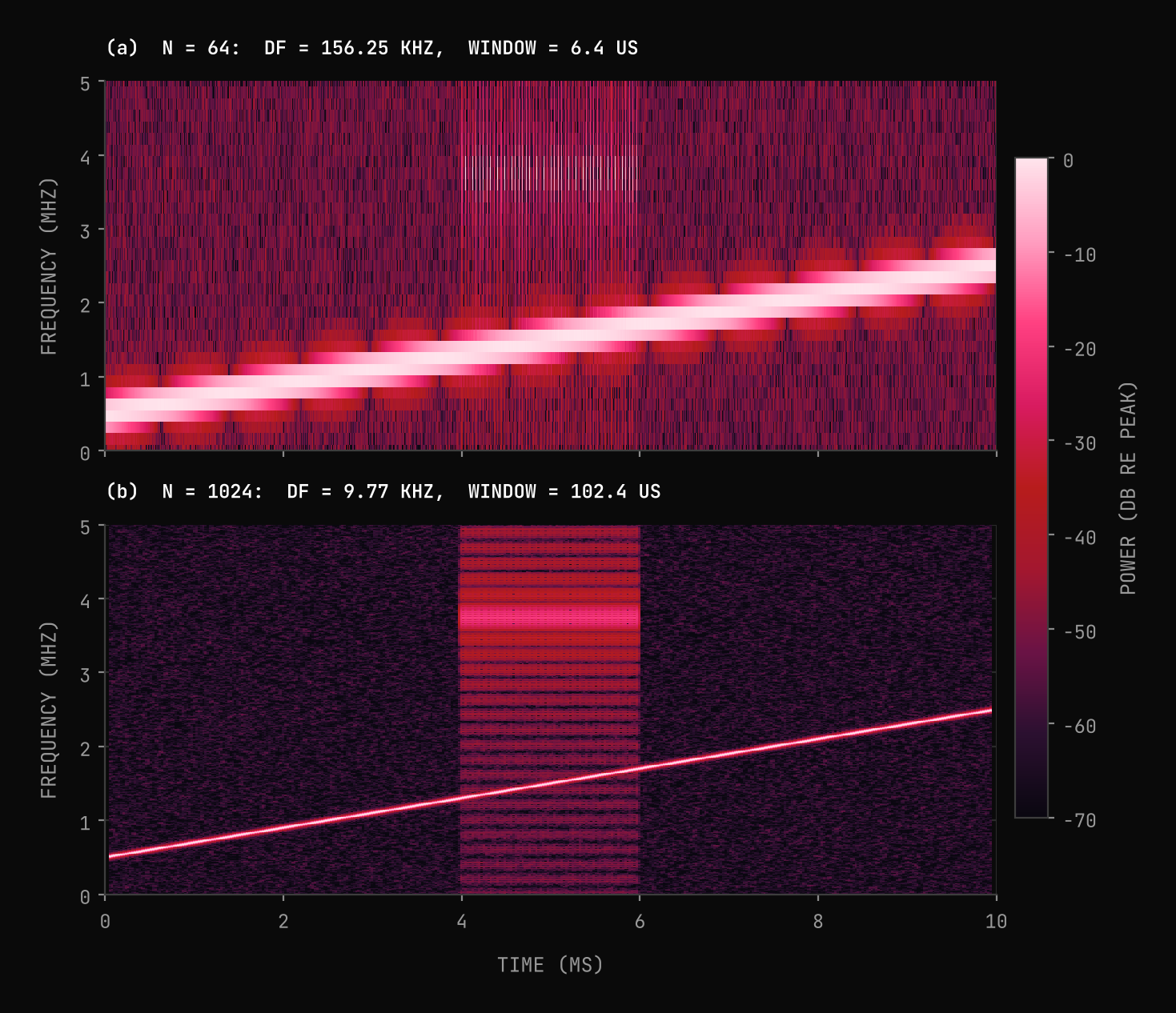
The numbers come from the script that drew the figure. At $N=64$ the bins are 156.25 kHz apart and the window is 6.4 µs long. The window is shorter than the 35 µs gap between pulses, so all 50 pulses show up as separate events. The cost is the chirp: measured at 2 ms, its line is 312.6 kHz wide between its $-6$ dB points.

At $N=1024$ the bins are 9.77 kHz apart and the window is 102.4 µs long. The chirp line narrows to 20.6 kHz, 15.2 times thinner, and the noise floor sits lower relative to the signal: each bin is 16 times narrower, so it admits 12.04 dB less noise relative to a steady tone. The cost is the burst: each window spans more than two pulse intervals, so the 50 pulses merge into one block whose level varies by only 0.6 dB. What this panel shows instead is the burst's spectrum, a set of lobes with nulls every 200 kHz, one over the 5 µs pulse width.

There is a second, smaller effect in panel (b). The chirp moves 200 MHz per second, so it sweeps 20.48 kHz during one 1024-sample window, about two bins. Make the window much longer and the chirp's own motion starts to widen the line again. For a moving signal there is a best window length, and it depends on the signal, not on the instrument.

By April 18 Fabric had one interface, a React front end talking to a Python service. That is a web application, not something an engineer can install. Chapter 6 covers the Tauri desktop wrapper that started on April 25, the packaging bugs that hid it, and what it took to ship. You can open the current scope, waterfall included, in Apexia Fabric in simulation today.